Working with spatial data from the portal
Source:vignettes/articles/spatial_data.Rmd
spatial_data.RmdThere is a ton of spatial data on the City of Toronto Open Data Portal.
Spatial resources are retrieved the same way as all other resources, by
using get_resource(), and may require the sf
package.
We can look at the locations of EarlyON
Child and Family Centres in Toronto. As the portal describes, these
centres offer free programs to caregivers and children, providing
programs to strengthen relationships, support education, and foster
healthy child development. The result of pulling this data in through
the package is an sf object with WGS84 projection.
library(opendatatoronto)
library(dplyr)

earlyon_centres <- search_packages("EarlyON Child and Family Centres") %>%
  list_package_resources() %>%
  filter(name == "EarlyON Child and Family Centres Locations - geometry - 4326.zip") %>%
  get_resource()
#> Reading layer `EarlyON Child and Family Centres Locations - geometry - 4326' from data source `/tmp/RtmpLxjINW/EarlyON Child and Family Centres Locations - geometry - 4326.shp'
#>   using driver `ESRI Shapefile'
#> Simple feature collection with 238 features and 34 fields
#> Geometry type: MULTIPOINT
#> Dimension:     XY
#> Bounding box:  xmin: -79.5969 ymin: 43.59448 xmax: -79.14021 ymax: 43.82965
#> Geodetic CRS:  WGS 84

earlyon_centres
#> Simple feature collection with 238 features and 34 fields
#> Geometry type: MULTIPOINT
#> Dimension:     XY
#> Bounding box:  xmin: -79.5969 ymin: 43.59448 xmax: -79.14021 ymax: 43.82965
#> Geodetic CRS:  WGS 84
#> # A tibble: 238 × 35
#>    X_id1 service2   agency3 loc_id4 program5 languag6 french_7 indigen8 program9
#>    <dbl> <chr>      <chr>     <dbl> <chr>    <chr>    <chr>    <chr>    <chr>
#>  1     1 City of T… Regent…   13650 101 Spr… NA       NA       NA       NA
#>  2     2 City of T… West N…   14380 1033 Ea… NA       NA       NA       NA
#>  3     3 City of T… West S…   12554 2555 Ea… NA       NA       NA       NA
#>  4     4 City of T… Macaul…   12562 2700 Du… NA       NA       NA       NA
#>  5     5 City of T… Regent…   13648 38 Rege… NA       NA       NA       NA
#>  6     6 City of T… Regent…   13649 402 Shu… NA       NA       NA       NA
#>  7     7 City of T… Aginco…   13960 4139 Sh… NA       NA       NA       NA
#>  8     8 City of T… Macaul…   12545 48 Rege… NA       NA       NA       NA
#>  9     9 City of T… The Ma…   12549 Abiona … NA       NA       NA       NA
#> 10    10 City of T… Access…   13544 Access … NA       NA       NA       NA
#> # ℹ 228 more rows
#> # ℹ 26 more variables: service10 <chr>, buildin11 <chr>, address12 <chr>,
#> #   full_ad13 <chr>, major_i14 <chr>, ward15 <dbl>, ward_na16 <chr>,
#> #   located17 <chr>, school_18 <chr>, lat19 <dbl>, lng20 <dbl>,
#> #   website21 <chr>, website22 <chr>, website23 <chr>, consult24 <chr>,
#> #   consult25 <chr>, email26 <chr>, contact27 <chr>, contact28 <chr>,
#> #   phone29 <chr>, contact30 <chr>, dropinH31 <chr>, registe32 <chr>, …
If we want to plot this data on a map of Toronto, a shapefile to map the different neighbourhoods of Toronto is also available from the portal:
neighbourhoods <- list_package_resources("https://open.toronto.ca/dataset/neighbourhoods/") %>%
  filter(name == "Neighbourhoods - 4326.zip") %>%
  get_resource()
#> Reading layer `Neighbourhoods - 4326' from data source
#>   `/tmp/RtmpLxjINW/Neighbourhoods - 4326.shp' using driver `ESRI Shapefile'
#> Simple feature collection with 158 features and 11 fields
#> Geometry type: POLYGON
#> Dimension:     XY
#> Bounding box:  xmin: -79.63926 ymin: 43.581 xmax: -79.11527 ymax: 43.85546
#> Geodetic CRS:  WGS 84

neighbourhoods[c("AREA_NA7", "geometry")]
#> Simple feature collection with 158 features and 1 field
#> Geometry type: POLYGON
#> Dimension:     XY
#> Bounding box:  xmin: -79.63926 ymin: 43.581 xmax: -79.11527 ymax: 43.85546
#> Geodetic CRS:  WGS 84
#> # A tibble: 158 × 2
#>    AREA_NA7                                                             geometry
#>    <chr>                                                           <POLYGON [°]>
#>  1 South Eglinton-Davisville ((-79.38635 43.69783, -79.38623 43.6975, -79.38639…
#>  2 North Toronto             ((-79.39744 43.70693, -79.39837 43.70673, -79.3986…
#>  3 Dovercourt Village        ((-79.43411 43.66015, -79.43537 43.65988, -79.4355…
#>  4 Junction-Wallace Emerson  ((-79.4387 43.66766, -79.43841 43.66696, -79.43819…
#>  5 Yonge-Bay Corridor        ((-79.38404 43.64497, -79.38502 43.64478, -79.3855…
#>  6 Bay-Cloverhill            ((-79.38743 43.66051, -79.39049 43.65986, -79.3906…
#>  7 Bendale-Glen Andrew       ((-79.26392 43.75175, -79.26505 43.75152, -79.2651…
#>  8 Downsview                 ((-79.46453 43.75014, -79.4643 43.75011, -79.46402…
#>  9 Oakdale-Beverley Heights  ((-79.51192 43.73457, -79.51154 43.73289, -79.5112…
#> 10 Avondale                  ((-79.40838 43.75362, -79.40839 43.75362, -79.4084…
#> # ℹ 148 more rows
Then, we can plot the EarlyON centres along with a map of Toronto:
library(ggplot2)

ggplot() +
  geom_sf(data = neighbourhoods) +
  geom_sf(data = earlyon_centres) +
  theme_void()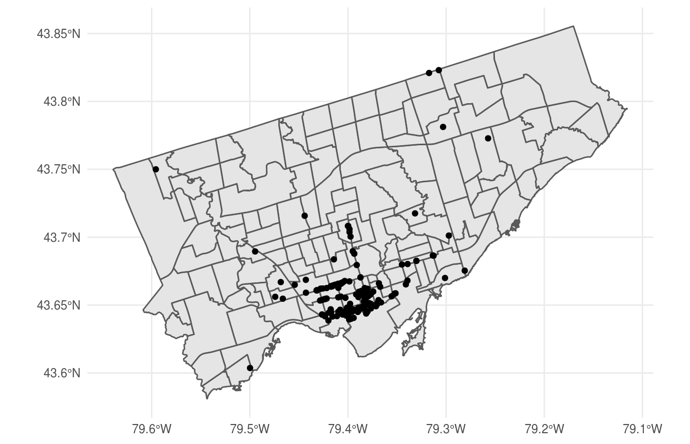
We may also wish to do something like analyze how many EarlyON
centres there are in each neighbourhood. We can count by neighbourhood,
using the sf package to join the two datasets, then
dplyr to summarise, and finally ggiraph to
create an interactive visualization, replacing geom_sf with
geom_sf_interactive and supplying a tooltip:
library(sf)
library(dplyr)
library(ggiraph)
library(glue)

earlyon_by_neighbourhood <- neighbourhoods %>%
  st_join(earlyon_centres) %>%
  group_by(neighbourhood = AREA_NA7) %>%
  summarise(n_earlyon = n_distinct(program5, na.rm = TRUE)) %>%
  mutate(tooltip = glue(("{neighbourhood}: {n_earlyon}")))

p <- ggplot() +
  geom_sf_interactive(data = earlyon_by_neighbourhood, aes(fill = n_earlyon, tooltip = tooltip)) +
  theme_void()

girafe(code = print(p))
This shows us, for example, that there are 9 EarlyON Centres in West Hill, 5 in Kensington-Chinatown, and 5 in South Riverdale:
earlyon_by_neighbourhood %>%
  as_tibble() %>%
  select(neighbourhood, n_earlyon) %>%
  arrange(-n_earlyon) %>%
  head()
#> # A tibble: 6 × 2
#>   neighbourhood                     n_earlyon
#>   <chr>                                 <int>
#> 1 West Hill                                 9
#> 2 Milliken                                  8
#> 3 Glenfield-Jane Heights                    7
#> 4 Kensington-Chinatown                      5
#> 5 Mount Olive-Silverstone-Jamestown         5
#> 6 South Riverdale                           5